Music Transcription with Convolutional Neural Networks (Jun 2016)

Note detection in music can be approached as an image recognition problem. Here I'll go over some of the differences between images of things like dogs and cars and images of music. I'll also describe techniques I used to modify neural networks from computer vision to produce sheet music transcriptions of (polyphonic) music that are actually quite playable.

Quick Introduction to Convolutional Networks

Convolutional neural networks (CNNs) have produced the most accurate results in computer vision for several years. In a typical CNN you start with an image as a 3 dimensional array (width, height, and 3 color channels) and then pass that data through several layers of convolutions, max pooling, and some kind of non-linearity, like a ReLU. The final layer outputs a score for each image class (flower, cat, etc.) representing the likelihood of the input belonging to that class. Backpropagation is used to iteratively update the convolution parameters from a set of labeled training data (pairs of input and desired output). This process builds up a sophisticated function composed of many simpler functions, primarily convolutions.

Images From Music

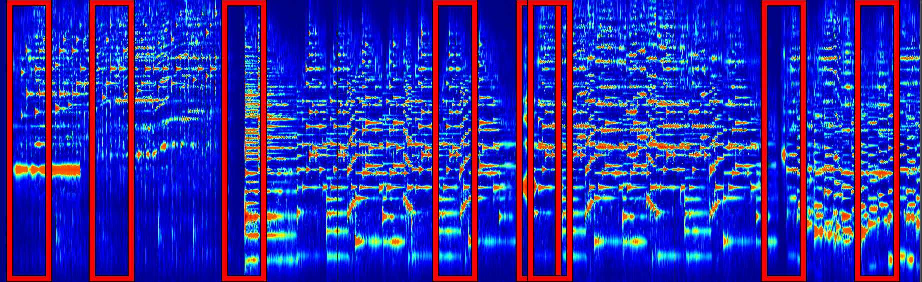
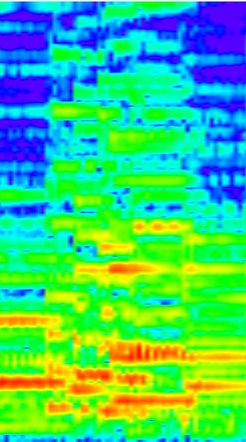
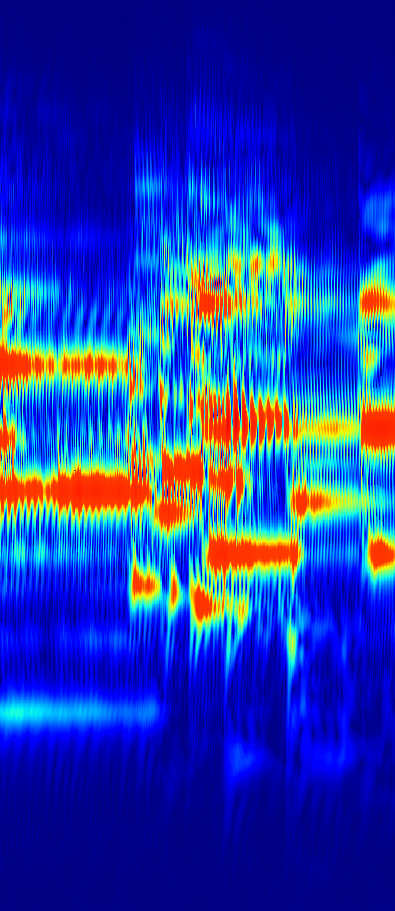
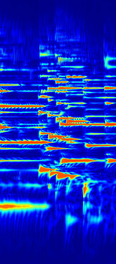
So, how is note detection in music similar to image recognition? It's possible to create images of audio called spectrograms. They show how the spectrum or frequency content changes over time. If you look at the left and right channels in stereo audio as analogous to the color channels in a photograph, then a spectrogram sort of resembles the 3 dimensional image array you'd feed into an image recognition neural network.

But how similar conceptually is finding notes in a spectrogram image to finding objects in a photograph? Music is simpler in the sense that there are not really any important textures to learn and spectrograms are usually composed of only two basic shapes: harmonics, which are narrowband, spanning a short frequency range and long time range, and drums or other wideband features, which span a short time range and long frequency range. There's also no rotation to worry about or zooming in and out at different distance scales. Furthermore, there's only one object class to detect: notes.

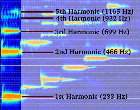
But a couple of aspects of notes are more challenging than images of physical objects. A note like B♭3 with a fundamental frequency of 233 Hz is composed of harmonics at multiples of that fundamental frequency, which tend to decrease in amplitude as you go up. So, unlike most physical objects, music notes aren't localized to a single region of the input.

Also unlike physical images, harmonics from different notes can interfere with each other. In photographs, one object can be partially hidden by another, but the object in front doesn't suffer any distortion. Notes do become distorted, though. Nearby harmonics can result in amplitude "beating", which you can see in the 4th and 5th harmonics in the image above. A note recognition algorithm needs to somehow take into account these aspects of music.

Using a CNN

Since I wanted to be able to detect multiple notes at once, I omitted the softmax layer usually used for classification. Instead of image classes there are simply 88 output nodes for each of the piano keys. Since it's not feasible to process the entire spectrogram image all at once, I first identified possible note start times and then took rectangular slices of the spectrogram centered at those times (the full frequency range and a fixed amount of time before and after to provide some context).

Note onsets are characterized by points where many frequencies increased in amplitude over some small time interval. A separate neural net could be trained to identify these locations, but I simply looked for local maxima in the mean amplitude change. It's ok if some of these points don't have any notes since the CNN will determine what specific notes are present, but it is bad to miss an area where there are notes. I trained the CNN to find which notes start in each region and ignored offsets. To create playable sheet music, I assume that every note ends when the next note begins.

Creating the Spectrogram

The Short Time Fourier Transform (STFT) is a common method for creating a spectrogram, but it has some downsides. The frequencies of the discrete Fourier Transform are spaced linearly, but musical note frequencies double with each octave (every 12 notes). I instead used something closer to the constant Q transform, a constant frequency to bandwidth ratio with 4 frequency bins per note. This works well for convolutions, since the distance between the 1st and 2nd harmonics or the 2nd and 3rd, etc. is now the same for all notes, independent of fundamental frequency. This means there's no need for fully connected layers and the CNN can be made entirely of convolutional and max pooling layers.

To reduce the interference effects from nearby harmonics, I increased the Q factor in regions where nearby harmonics were detected when generating the spectrogram. This is analogous to increasing the window size in the FFT, except it was only applied to a narrow frequency and time range. A higher Q reduces amplitude distortion from nearby harmonics, but the improved frequency resolution comes at the cost of poorer time resolution, so it's better to use a low Q factor by default to preserve information about how the amplitude changes in time. I also performed some non-linear scaling to get something closer to the log of the amplitude.

Adapting the CNN for Music

Since notes aren't localized to a single region and the CNN will need to look at the entire spectrum to determine whether any given note is present, I made most of the convolutions long and skinny, alternating between time and frequency dimensions: an Mx1 followed by a 1xN. These long convolutions helped efficiently connect distant regions of the spectrum. By the final layer, every output neuron is influenced by every input bin.

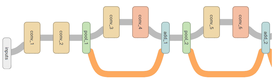
I also used the forward skip connections described in Microsoft's ResNet, which won the ILSVRC challenge in 2015. They help the network train faster and allow the output to be composed of a series of additions (residuals) on the input. This makes a lot of sense in music, where the output is essentially equivalent to the input after removing the non-fundamental harmonics.

Post-Processing

To boost the accuracy, additional processing was applied on the output of the CNN that filtered out some of the the lower confidence notes (notes with greater than 0.5 probability but less than some threshold). This involved a separate note detection algorithm, which used a more traditional approach of searching for peaks in the spectrogram, forming tracks of sequential peaks, and ordering candidate notes from most to least likely. The main idea behind this secondary algorithm is that the strongest track at any instant is very likely to be a low harmonic: a 1st, 2nd, or 3rd.
Update: I removed the post-processing in version 3.0.0, so only the CNN is used.

Training and Results

To train the network, I created a dataset of 2.5 million training examples from 3,000 MIDI files spanning several different genres of music. MIDI files contain information about the notes and instruments in the song, which makes it easy to create labeled truth data. A MIDI-to-WAV utility created the actual audio data used for spectrogram generation. The dataset had an average of 3 notes per training example.

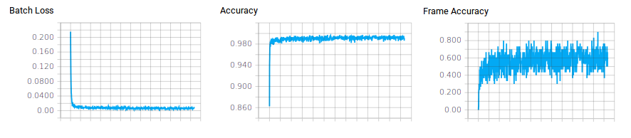
After training for a few days on a 980 Ti GPU in TensorFlow, the CNN had an accuracy of 99.200% on the evaluation split (data not used for training) at the note level. This number comes from rounding each of the 88 outputs to 0 or 1 and measuring the fraction of all outputs that matched the truth values. However, since the dataset had an average of 3 notes and 85 non-notes per training example, if the CNN never detected any notes it would be accurate 96.6% of the time with this measurement. I also measured the percentage of samples in the evaluation split where every single one of the 88 rounded outputs was correct. That came out to 60.326%. The accuracy of the entire end-to-end algorithm also depends on the accuracies of the onset time detection and filtering of the CNN’s output. For piano, only evaluating note starts and pitches, it achieves F-scores around 0.8.

You can download and try out this software yourself. The program generates musicXML files, which you can view and edit with any music notation program.